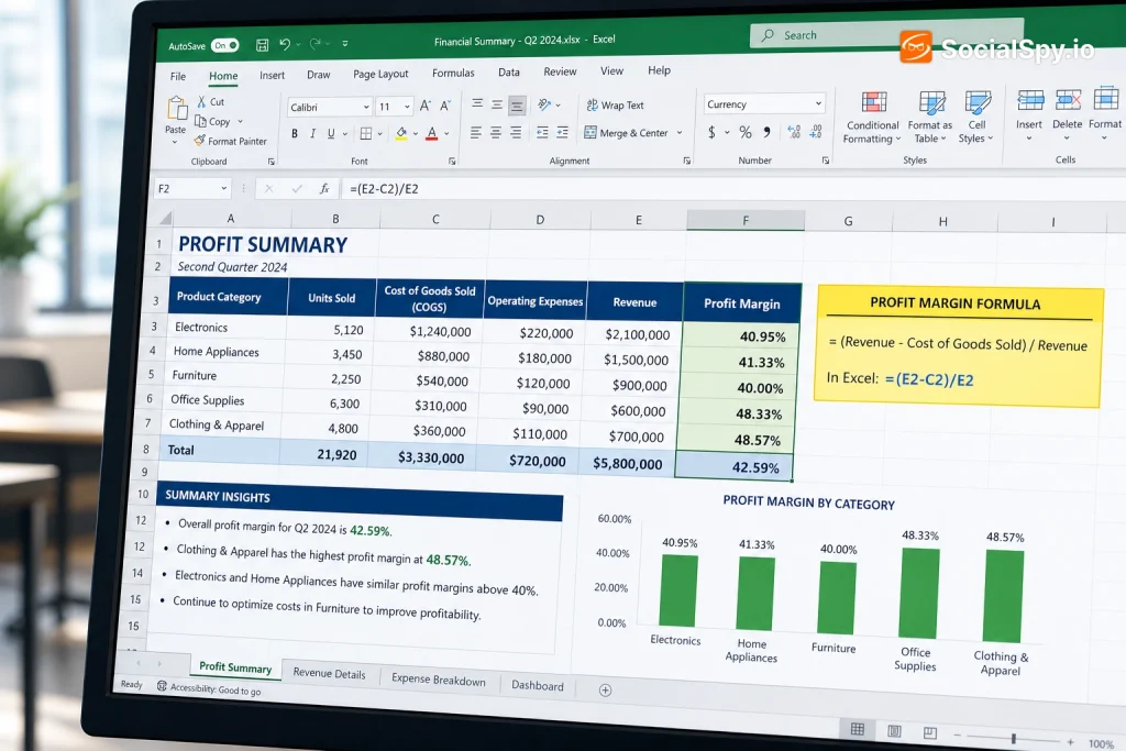
Every finance team, small business owner, and side-hustler eventually needs to answer one question fast: how much am I actually keeping after costs? Excel makes that calculation trivial once you know the right formula structure, but most people either hardcode numbers wrong or confuse gross margin with net margin. This guide breaks down the exact formulas, cell references, and formatting tricks to build a profit margin tracker that won’t break the moment you add a new product line.
The Core Formula, Explained
Profit margin measures how much of every dollar in revenue you actually keep after expenses. The universal structure in Excel is straightforward:
Profit Margin = (Revenue − Cost) / Revenue
In practice, that means if column B holds revenue and column C holds total cost, your formula in cell D2 looks like this: `=(B2-C2)/B2`. Once entered, you need to format the cell as a percentage (Home tab → Number Format → Percentage) or Excel will show a decimal like 0.35 instead of 35%.
Here’s why this trips people up: “cost” isn’t one fixed number. Depending on which costs you subtract, you get a completely different margin metric, and mixing them up leads to wildly inaccurate business decisions.
- Gross margin subtracts only the cost of goods sold (COGS)
- Operating margin subtracts COGS plus operating expenses (rent, salaries, marketing)
- Net margin subtracts everything — COGS, operating costs, interest, and taxes
A retailer with a 60% gross margin might have a net margin of just 8% once payroll and overhead are factored in. Both numbers are “correct” — they just answer different questions.
Building Each Margin Type in Excel
Let’s set up a realistic spreadsheet structure so you can see how the formulas actually differ once you separate expense categories.
Sample Layout
| Column | Contents |
|---|---|
| A | Product/Period name |
| B | Revenue |
| C | COGS |
| D | Operating Expenses |
| E | Taxes & Interest |
Formulas for Each Metric
- Gross Profit Margin: `=(B2-C2)/B2` — measures production efficiency before overhead
- Operating Margin: `=(B2-C2-D2)/B2` — reveals how well the core business runs day-to-day
- Net Profit Margin: `=(B2-C2-D2-E2)/B2` — the bottom-line figure investors and lenders actually care about
Notice the pattern: each formula just adds one more subtraction inside the parentheses while keeping the same denominator (revenue). This consistency is intentional — it lets you build all three metrics side by side in adjacent columns without rewriting logic each time.
A common mistake is dividing by the wrong figure — for instance, dividing net profit by COGS instead of revenue, which inflates the percentage and misleads anyone reading the report. Always keep revenue as your denominator unless you’re deliberately calculating a markup formula instead, which is a different metric entirely (markup divides by cost, margin divides by revenue).
Making the Formula Scalable Across Rows and Sheets
A single-row formula is only useful once. The real value comes when you drag it across dozens of products, months, or business units without manually retyping anything.
Once you’ve built the formula in row 2, you can drag the fill handle down or use Excel’s copy shortcuts to replicate it instantly across your entire dataset. If you’re unfamiliar with the fastest ways to do this without breaking cell references, the guide on Excel copy formula techniques covers keyboard shortcuts and fill-handle tricks that save real time on large spreadsheets.
Here’s where relative vs. absolute references matter enormously:
- Use relative references (like `B2`) when each row has its own unique revenue and cost — this lets the formula shift automatically as you copy it down
- Use absolute references (like `$B$1`) when you’re referencing a fixed value, such as a company-wide tax rate applied to every row
- Mixed references (`$B2` or `B$2`) lock only the column or row, useful when building margin comparison tables across multiple periods
For example, if cell F1 holds a flat corporate tax rate you’re applying to every product line, your net margin formula might become `=(B2-C2-D2-(B2-C2-D2)*$F$1)/B2` — the dollar signs anchor F1 so it doesn’t shift when copied to row 20.
Common Errors and How to Fix Them
Excel profit margin formulas break in predictable ways. Knowing these failure points ahead of time saves hours of debugging a spreadsheet that “just shows weird numbers.”
Industry analysts who train small business owners on financial modeling consistently point to #DIV/0! errors and formatting mistakes as the two most common issues in profit margin spreadsheets — not calculation logic.
#DIV/0! Error This happens when revenue is zero or the cell is blank. Wrap your formula in an `IFERROR` function to keep the sheet clean:
`=IFERROR((B2-C2)/B2,”N/A”)`
Negative Margins Displaying Incorrectly If costs exceed revenue, the result is negative — which is accurate, but make sure your percentage formatting doesn’t hide the negative sign. Custom formatting like `0.0%;[Red]-0.0%` displays losses in red for quick visual scanning.
Decimal vs. Percentage Confusion The most frequent beginner mistake is manually multiplying by 100 inside the formula (`=(B2-C2)/B2100`) and then also applying percentage formatting, which doubles the value. Pick one method: either format the cell as a percentage and skip the `100`, or leave it as a raw number and label the column “Margin (%)” manually.
Mixing Up Which Column Is Cost When COGS and operating expenses sit in adjacent columns, it’s easy to reference the wrong one. Naming your columns clearly and using Excel’s named ranges (Formulas tab → Define Name) reduces this risk substantially, especially in shared workbooks where multiple people edit the sheet.
Advanced Techniques for Margin Analysis
Once the basic formula works, most finance-savvy users push further — building dashboards, conditional formatting alerts, and multi-product comparisons that reveal trends a single number can’t show.
Conditional Formatting for Margin Health
Rather than reading a column of percentages manually, apply Home → Conditional Formatting → Color Scales to your margin column. This instantly flags underperforming products in red and strong performers in green — useful when scanning 200+ SKUs in a retail spreadsheet.
Weighted Average Margin Across Products
A simple average of margin percentages across products is misleading if products have vastly different revenue volumes. The correct approach uses SUMPRODUCT:
`=SUMPRODUCT(B2:B20,D2:D20)/SUM(B2:B20)`
This weights each product’s margin by its revenue contribution, giving a far more accurate blended margin than a plain `AVERAGE()` function would.
Combining Text Labels with Margin Data
When building executive summary tabs, it’s common to merge a product name with its margin percentage into a single readable string — like “Widget A: 34.2% margin” — for a cleaner report output. The techniques covered in how to combine text from two cells in Excel apply directly here, letting you use `CONCAT` or the `&` operator alongside `TEXT()` to format the percentage inline.
Sorting Products by Profitability
Once your margin column is built, ranking products from most to least profitable helps prioritize inventory and marketing decisions. Excel’s newer dynamic array functions make this far easier than manual sorting — the breakdown on the SORT Excel function shows how to auto-rank an entire product list by margin percentage with a single formula that updates live as new data comes in.
Building a Reusable Margin Dashboard Template
For anyone tracking margins monthly or quarterly, a one-off formula isn’t enough — you want a template that updates itself as new data flows in.
Here’s a practical structure that scales well:
- Raw data tab — revenue, COGS, opex, and taxes entered per product/period, never manually edited elsewhere
- Calculations tab — all margin formulas referencing the raw data tab, using absolute references for shared assumptions like tax rate
- Dashboard tab — pulls summary figures using `INDEX/MATCH` or `XLOOKUP`, displays via charts and conditional formatting
- Notes column — a text field explaining anomalies (e.g., “Q3 margin dropped due to shipping cost spike”)
Keeping raw data physically separate from calculations is the single biggest habit that prevents spreadsheet errors down the line. When formulas and inputs live in the same cells, someone inevitably overwrites a formula with a hardcoded number, and the whole sheet’s integrity breaks silently.
For polish, many users also standardize header formatting — this is where knowing how to change text case in Excel comes in handy, since converting inconsistent column headers (like “revenue” vs. “Revenue” vs. “REVENUE”) into a uniform case makes the dashboard look professional and prevents lookup functions from failing due to case-sensitive mismatches in some formula contexts.
Conclusion
The profit margin formula itself is genuinely simple — subtract cost from revenue, divide by revenue, format as a percentage. What separates a functional spreadsheet from a fragile one is everything around that formula: correct cost categorization, absolute vs. relative references, error handling with `IFERROR`, and keeping raw data separate from calculations. Build it once with these principles in 2026, and you’ll have a margin tracker that scales from five products to five hundred without a rebuild.
FAQ
Profit margin divides profit by revenue (`=(B2-C2)/B2`), while markup divides profit by cost (`=(B2-C2)/C2`). They produce different percentages for the same numbers — a $50 cost item sold for $100 has a 50% margin but a 100% markup — so always confirm which metric a stakeholder is actually asking for before building the formula.
This usually happens when the formula references the wrong column, dividing by cost instead of revenue, or when cost figures are entered as negative numbers and the subtraction effectively adds them back. Double-check that your denominator is genuinely the revenue cell and that cost values are entered as positive numbers before troubleshooting further.
Yes, if your raw data comes from an external source like a POS system or accounting software, you can import it via Power Query or a simple CSV import, then apply the margin formula once and drag it down — Excel will calculate margins for hundreds of rows instantly as long as the revenue and cost columns stay consistent.