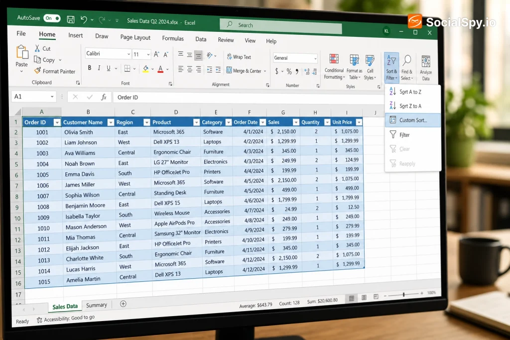
Microsoft’s SORT function quietly changed how millions of people organize spreadsheet data, replacing manual drag-and-drop reordering with a single dynamic formula that updates itself automatically. If you’re still right-clicking column headers and choosing “Sort A to Z” every time your data changes, you’re doing more work than necessary in 2026’s version of Excel.
What the SORT Function Actually Does
SORT is part of Excel’s dynamic array family, introduced alongside FILTER, UNIQUE, and XLOOKUP starting with Microsoft 365 subscriptions. Unlike the classic Sort dialog box under the Data tab, SORT is a live formula. It spills results into adjacent cells and refreshes the moment your source data changes — no re-clicking required.
The function takes up to four arguments, and only the first one is mandatory.
| Argument | Required? | What It Does |
|---|---|---|
| array | Yes | The range or array you want sorted |
| sort_index | No | Which row or column number to sort by (default is 1) |
| sort_order | No | 1 for ascending (default), -1 for descending |
| by_col | No | FALSE sorts by row (default), TRUE sorts by column |
A basic formula looks like `=SORT(A2:A20)`, which sorts a single column ascending. Add a second argument for descending order, like `=SORT(A2:A20,1,-1)`, and Excel flips the order instantly.
Early adopters of dynamic arrays reported cutting spreadsheet maintenance time significantly because sorted views no longer needed manual refreshing after every data entry.
SORT vs. the Traditional Data > Sort Command
This is where most confusion happens, because Excel now offers two completely different ways to sort data that look similar but behave very differently under the hood.
Key Differences
- Data modification: The classic Data > Sort command physically rearranges your original rows. SORT the function leaves source data untouched and creates a new, separate output.
- Dynamic updates: A traditional sort is a one-time action — if you add a new row, you must sort again. SORT recalculates automatically, similar to how SUM or VLOOKUP behave.
- Spill behavior: SORT uses the spill range feature, meaning one formula in one cell can populate dozens of cells below and beside it. Editing any single cell inside a spill range triggers a #SPILL! error unless you edit the anchor cell.
- Formula auditing: Because SORT is a formula, you can nest it inside other functions like FILTER or INDEX, something impossible with the button-based sort.
When Each Method Makes More Sense
| Scenario | Best Tool |
|---|---|
| One-time cleanup of a static report | Data > Sort |
| Live dashboard that updates as data comes in | SORT function |
| Sorting a Table with filters applied | Data > Sort (works natively with Table filters) |
| Combining sorting with filtering logic | SORT nested with FILTER |
| Sorting data you don’t want to permanently rearrange | SORT function |
Practical Examples Every Excel User Should Know
The real value of SORT shows up once you move past single-column examples into scenarios that mirror actual work — sales reports, inventory lists, and survey results.
- Sort a single column ascending: `=SORT(B2:B50)` — ideal for alphabetizing a list of customer names without touching the original table.
- Sort descending by a specific column: `=SORT(A2:D50,3,-1)` sorts an entire four-column range using column 3 (say, revenue) from highest to lowest.
- Sort by multiple columns: Using an array constant like `=SORT(A2:D50,{1,2},{1,-1})` sorts first by column 1 ascending, then by column 2 descending — useful for sorting by region, then by sales within each region.
- Sort horizontally: `=SORT(A1:F1,1,1,TRUE)` reorders a single row of values left to right, which comes up in transposed datasets or timeline layouts.
- Combine with UNIQUE: `=SORT(UNIQUE(A2:A200))` produces a clean, alphabetized list of distinct values in one step — a favorite among analysts building dropdown lists for data validation.
- Sort by a helper column that isn’t displayed: You can reference a hidden ranking column as the sort_index, letting you sort by criteria the viewer never sees in the final output.
These examples work identically in Excel for Windows, Excel for Mac, and Excel on the web, as long as your subscription includes dynamic array support.
Common Errors and How to Fix Them
Dynamic arrays introduce a new category of error messages that didn’t exist in older Excel versions, and they trip up even experienced users.
- #SPILL!: Appears when something is blocking the range where results need to spill — usually leftover data in cells below your formula. Clear the blocking cells and the error resolves instantly.
- #CALC!: Occurs when the sorted array would return zero items, often because a nested FILTER found no matching rows.
- #NAME?: Shows up if you’re using an older Excel version (like Excel 2016 or Excel 2019) that doesn’t recognize SORT at all — this function requires Microsoft 365 or Excel 2021 and later.
- #VALUE!: Typically caused by mismatched array sizes in the sort_index or sort_order arguments, such as providing two sort columns but only one sort order.
- Wrong sort_index reference: A frequent mistake is forgetting that sort_index refers to the column’s position within the selected array, not its actual worksheet column letter.
If you inherited a spreadsheet showing #NAME? errors where SORT should be working, check the Microsoft 365 version number under File > Account before assuming the formula is broken.
Advanced Techniques: Nesting SORT with Other Functions
Power users rarely use SORT alone. Its real strength emerges when it’s layered with FILTER, INDEX, and XLOOKUP to build fully automated reporting systems.
Combining SORT and FILTER
A common pattern is `=SORT(FILTER(A2:D500,C2:C500>1000),3,-1)`, which filters a sales table for orders above $1,000, then sorts the results by column 3 in descending order — all in a single cell. This eliminates the need for separate filter and sort steps, and the output updates live as new rows are added to the source table.
Building a Top 10 List
Analysts frequently pair SORT with INDEX to extract ranked lists:
- `=INDEX(SORT(A2:B100,2,-1),SEQUENCE(10),{1,2})` returns just the top 10 rows after sorting the full range by column 2.
- This avoids manually copying data into a separate “Top 10” tab that needs constant updating.
SORTBY: The More Flexible Sibling
Excel also offers SORTBY, a related function that sorts one array based on values in a completely different array — useful when the sort criteria isn’t part of the data you want displayed.
| Feature | SORT | SORTBY |
|---|---|---|
| Sort criteria location | Must be within the array itself | Can be a completely separate array |
| Multiple sort keys | Yes, via array constants | Yes, natively supports multiple pairs |
| Best for | Simple in-place reordering | Sorting by a hidden or external ranking |
| Syntax complexity | Lower | Slightly higher |
For instance, `=SORTBY(A2:A50,B2:B50,-1)` sorts a list of product names (column A) based on sales figures in column B, without needing sales figures to appear in the output at all.
Version Availability and Platform Support in 2026
Not every Excel installation supports SORT, and this remains the single biggest source of user frustration reported in Microsoft community forums.
| Platform | SORT Function Support |
|---|---|
| Microsoft 365 (Windows/Mac) | Fully supported |
| Excel 2021 (perpetual license) | Fully supported |
| Excel 2024 (perpetual license) | Fully supported |
| Excel 2019 and earlier | Not supported — returns #NAME? |
| Excel for the web | Fully supported |
| Excel mobile apps (iOS/Android) | Fully supported |
| Google Sheets | Supported via its own SORT function with similar but not identical syntax |
Microsoft 365 subscriptions currently run roughly $70 per year for Personal plans and $100 per year for Family plans as of 2026 pricing, and both tiers include full dynamic array functionality. Perpetual-license buyers purchasing Excel 2024 as a one-time purchase also get SORT, but they miss out on newer AI-assisted features Microsoft continues rolling out to subscribers only.
- If your organization is still running Excel 2016 or 2019 under a volume license, SORT formulas shared by colleagues will break entirely when opened.
- IT departments migrating large enterprises to Microsoft 365 often cite dynamic array compatibility as a key driver, since finance teams increasingly build models around SORT and FILTER.
- Google Sheets users should note that its SORT function uses a different argument order — `SORT(range, sort_column, is_ascending)` — meaning formulas aren’t directly portable between the two platforms without editing.
Conclusion
The SORT function represents a genuine shift in how spreadsheet logic gets built — away from manual, repeatable clicks and toward self-maintaining formulas that behave more like small programs than static commands. For anyone building recurring reports, dashboards, or shared models where data keeps changing, learning SORT (and its sibling SORTBY) pays back the initial learning curve within the first few uses. The bigger strategic point for 2026 is version compatibility: as Microsoft continues pushing AI features exclusively to Microsoft 365 subscribers, organizations clinging to older perpetual licenses will find themselves increasingly locked out of formulas like SORT that colleagues elsewhere take for granted. If you manage spreadsheets that get shared across teams, confirming everyone’s Excel version supports dynamic arrays should happen before you build a single SORT formula into a shared workbook.
FAQ
No, SORT never alters the source range. It creates a new spilled array of results in a separate location, leaving your original data exactly as it was, which makes it safer for shared workbooks where multiple people reference the same source table.
This almost always means your version of Excel doesn’t support dynamic array functions. SORT requires Microsoft 365, Excel 2021, or Excel 2024; older perpetual versions like Excel 2016 or 2019 will reject the formula and display #NAME? instead of a result.
SORT reorders an array using a column that exists within that same array, while SORTBY can reorder an array based on values from a completely separate range that never even appears in the output. Use SORT for straightforward reordering and SORTBY when your ranking criteria lives somewhere else in the spreadsheet, like a hidden priority score column.