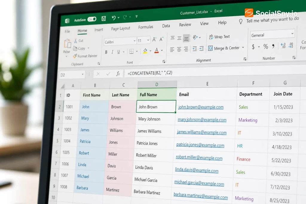
Combining text from two cells is one of those Excel tasks everyone eventually needs, whether you’re merging first and last names, building full addresses from separate fields, or stitching together product codes. Excel actually gives you four or five different ways to do it, and picking the right one depends on whether you need the result to update automatically, how much formatting control you want, and whether you’re comfortable typing formulas at all.
The Four Main Ways to Combine Cells in Excel
Excel offers several distinct methods, and none of them is objectively “best” — each fits a different scenario. Before diving into syntax, it helps to see them side by side.
| Method | Best For | Multiple Cells at Once? |
|---|---|---|
| Ampersand (&) | Quick two-cell joins | Yes, but gets clunky |
| CONCAT function | Modern replacement for CONCATENATE | Yes |
| TEXTJOIN function | Joining with a shared delimiter | Yes, very efficiently |
| Flash Fill | No-formula, pattern-based merging | Yes, automatically |
A few things worth knowing upfront:
- CONCATENATE is the original merging function, but Microsoft has officially marked it as a legacy function — it still works, but it won’t get updates and isn’t recommended for new spreadsheets.
- TEXTJOIN, introduced in Excel 2019 and included in every Microsoft 365 subscription since, is generally considered the modern standard because it lets you specify a delimiter once instead of retyping it between every cell.
- Flash Fill requires zero formula knowledge and is arguably the most underused feature in all of Excel.
- All formula-based methods produce a live result that updates if the source cells change; Flash Fill does not.
Industry surveys of spreadsheet users consistently find that fewer than half of everyday Excel users know TEXTJOIN exists, even though it was added years ago — most people default to the ampersand out of habit.
Using the Ampersand (&) Operator
The ampersand is the simplest and most universally compatible method — it’s worked since the earliest versions of Excel and will work in every version going forward.
Here’s the basic pattern for combining two cells, say A2 (first name) and B2 (last name):
- Click an empty cell where you want the combined result to appear.
- Type `=A2&” “&B2` and press Enter.
- Excel joins the two values with a single space between them.
- Drag the fill handle down to apply the same formula to other rows.
Notice the `” “` in the middle — that’s a literal space character wrapped in quotes. Without it, “John” and “Smith” would merge into “JohnSmith” with no space at all.
You can swap that space for anything you want:
- `=A2&”, “&B2` produces “Smith, John” style formatting
- `=A2&”-“&B2` produces “A123-B456” for product codes
- `=A2&” (“&B2&”)”` produces “John (Smith)” with parentheses
One limitation worth flagging: once you start combining four, five, or six cells with the ampersand, the formula gets long and easy to mistype, since you need a separate `&”delimiter”&` between every single cell reference.
TEXTJOIN and CONCAT: The Modern Approach
TEXTJOIN solves the “too many ampersands” problem by letting you define the delimiter exactly once, then list all the cells you want joined afterward.
The syntax looks like this:
=TEXTJOIN(delimiter, ignore_empty, text1, [text2], …)
Breaking down each argument:
- delimiter — the character(s) to insert between values (a space, comma, hyphen, etc.)
- ignore_empty — TRUE or FALSE; setting this to TRUE skips blank cells instead of adding extra delimiters
- text1, text2… — the cells or ranges you want combined
A real example: `=TEXTJOIN(“, “, TRUE, A2:D2)` combines everything in the range A2 through D2 with a comma-and-space between each value, automatically skipping any blank cells in that range. That last part matters — with the plain ampersand method, a blank cell still produces an awkward double-comma or double-space in your output.
CONCAT is TEXTJOIN’s simpler sibling. It joins multiple cells or ranges without a custom delimiter option:
- `=CONCAT(A2:D2)` mashes everything together with nothing in between
- `=CONCAT(A2,” “,B2)` still works if you manually insert separators
- Microsoft designed CONCAT as the direct successor to CONCATENATE, and it also supports entire ranges, which CONCATENATE never could
For most real-world merging tasks — names, addresses, IDs — TEXTJOIN is the better default because the ignore_empty argument alone saves significant cleanup time on messy spreadsheets.
Flash Fill: No Formulas Required
Flash Fill is Excel’s pattern-recognition feature, and it’s genuinely one of the fastest ways to merge cells if you don’t want to think about syntax at all.
Here’s how it works in practice:
- In a new column, type out what you want the combined result to look like for the first row (e.g., type “John Smith” next to the row containing “John” in one column and “Smith” in another).
- Press Enter, then start typing the second row’s expected result.
- Excel usually detects the pattern after two or three examples and shows a preview of the rest, grayed out.
- Press Enter or Ctrl+E to accept the entire filled column.
Flash Fill is fast, but it comes with real tradeoffs:
- It produces static text, not a formula — if the original data changes, Flash Fill results do not update automatically.
- It works best on clean, consistent data; irregular formatting or inconsistent spacing can confuse the pattern detection.
- It’s found under Data > Flash Fill, or triggered instantly with the keyboard shortcut Ctrl+E.
- It doesn’t work at all in older Excel versions before 2013.
If you’re merging data once for a report and never touching it again, Flash Fill is arguably faster than typing any formula. If the spreadsheet is a living document that gets updated weekly, stick with TEXTJOIN or the ampersand so your combined column stays accurate automatically. This same logic — formulas for anything that needs to stay current, static tools for one-off snapshots — comes up constantly in spreadsheet work, similar to how choosing between Excel’s copy formula shortcuts versus manual retyping depends on whether your source data is going to keep changing.
Common Mistakes and How to Fix Them
Most problems people run into when combining cells fall into a handful of predictable categories.
Missing or Extra Spaces
This is by far the most common complaint. Typing `=A2&B2` without a space character produces “JohnSmith” jammed together with no gap.
Fix it by explicitly inserting `” “` between the references: `=A2&” “&B2`. If you’re combining more than two cells with TEXTJOIN, remember the delimiter argument handles spacing for you automatically, so you don’t need to add extra quotation marks manually.
Numbers Turning Into Unexpected Text
When you combine a number-formatted cell with a text cell, the result becomes plain text — meaning you can no longer do math on it, and formatting like currency symbols or decimal places can disappear.
For example, if B2 contains the number 5000 formatted as currency ($5,000.00), a simple `=A2&” “&B2` will output “Product 5000″ — the dollar sign and comma vanish because ampersand concatenation converts everything to raw text. To preserve formatting, wrap the number in the TEXT function: `=A2&” “&TEXT(B2,”$#,##0.00”)` keeps the currency formatting intact in the merged string.
Formulas Breaking When Rows Are Inserted or Deleted
If you insert a new row above your data range, formula-based merges usually adjust correctly since Excel updates cell references automatically. But Flash Fill results won’t move or recalculate at all, since they’re static text — this is one of the biggest hidden risks of relying on Flash Fill for data that changes structure over time.
Combining Dates Incorrectly
Dates stored as cell values are actually serial numbers behind the scenes, so `=A2&” “&B2` on a date cell often spits out something like “45678” instead of “8/15/2026.” The fix is the same TEXT function trick: `=A2&” “&TEXT(B2,”mm/dd/yyyy”)` forces Excel to display the readable date format inside your combined text.
Practical Real-World Examples
Seeing these formulas applied to actual scenarios makes the syntax click faster than staring at abstract placeholders.
Merging First and Last Names `=A2&” “&B2` turns “Sarah” and “Johnson” into “Sarah Johnson.” This is easily the single most searched Excel merging task, common when importing contact lists from a CRM or email platform.
Building Full Mailing Addresses `=TEXTJOIN(“, “, TRUE, A2:D2)` where columns hold street, city, state, and zip produces a clean “123 Main St, Springfield, IL, 62704” — and the TRUE argument means if the “state” column happens to be blank for an international address, it skips it instead of leaving a stray comma.
Creating Unique Product SKUs `=A2&”-“&B2&”-“&C2` combining category, size, and color codes might generate “SHIRT-M-BLU” from three separate reference columns — useful for inventory systems that need machine-readable identifiers built from human-readable fields.
Combining Cells With Line Breaks `=A2&CHAR(10)&B2` inserts an actual line break between two values instead of a space, which is handy for label printing or mailing merges — though you’ll need to enable Wrap Text on the cell for the break to display visually rather than showing as a strange gap.
Adding Conditional Text `=A2&” — “&IF(B2=””,”No Notes”,B2)` combines a name with a notes field, but substitutes “No Notes” whenever the second cell is empty, avoiding an awkward trailing dash with nothing after it.
Once your combined-text column is built, you’ll often want to sort or filter based on that new data — this is where features like Excel’s SORT function become genuinely useful, letting you reorder merged names or SKUs alphabetically without disturbing the original source columns.
Conclusion
There’s no single “correct” way to combine text from two cells — the right choice depends entirely on context. If you’re doing a quick one-off merge on data that will never change, Flash Fill (Ctrl+E) genuinely is the fastest path and doesn’t require remembering any syntax. But for spreadsheets that get updated regularly — customer lists, inventory sheets, ongoing reports — a live formula is worth the extra typing because it keeps your combined column accurate automatically whenever the source data shifts.
Between the formula options, the ampersand is fine for simple two-cell jobs, but TEXTJOIN has quietly become the better default for anything involving three or more cells, ranges, or messy data with occasional blanks. Learning the TEXT function alongside it — to preserve number and date formatting — will save you from the single most common merging headache. Master these together and you’ll rarely need to look up “how to combine cells in Excel” again.
FAQ
CONCATENATE is the older function that Microsoft now classifies as legacy — it still works for backward compatibility but only accepts individual cell references, not entire ranges. CONCAT is its modern replacement, supports both individual cells and full ranges like A2:D2, and is the version Microsoft recommends using going forward, though it still lacks the custom delimiter option that makes TEXTJOIN more powerful.
This usually happens when you merge a formatted number or date without using the TEXT function first, since concatenation converts values to their raw underlying form — a date becomes a serial number and currency loses its dollar sign and commas. Wrapping the numeric cell in TEXT(cell, “format code”), such as TEXT(B2,”$#,##0.00″) for currency or TEXT(B2,”mm/dd/yyyy”) for dates, forces Excel to keep the readable formatting inside the combined text.
Yes, and TEXTJOIN is specifically built for this — a formula like =TEXTJOIN(“, “, TRUE, A2:F2) merges every cell in that six-column range with a comma separator in a single step. The ampersand method also works for multiple cells, but it requires manually typing an “&” between every single reference, which becomes error-prone once you’re combining more than three or four cells.