Rotating a dataset from rows to columns (or vice versa) used to mean rebuilding an entire spreadsheet by hand, cell by cell. Excel actually has several built-in tools for this exact problem, ranging from a one-click paste option to a dynamic formula that updates automatically. Knowing which method fits your situation can save you hours on messy reports, survey exports, and pivoted data dumps.
What “Transpose” Actually Means in Excel
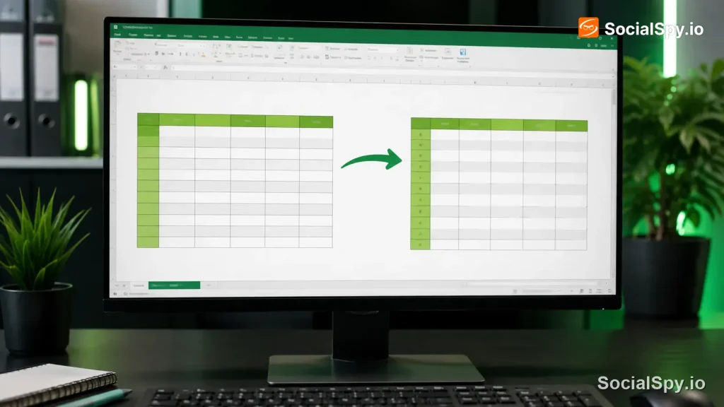
Transposing simply flips the orientation of your data. Rows become columns, and columns become rows, so the cell that was in row 3, column B moves to row 2, column D (or wherever the new layout places it).
This comes up constantly in real work scenarios:
- A survey export lists questions across columns and respondents down rows, but you need respondents across the top for a comparison table.
- A finance report has months running horizontally, but your dashboard template expects them vertically.
- A dataset pulled from a database or CSV file has the wrong axis for a chart you’re trying to build.
- You’ve inherited a spreadsheet from a colleague who structured it “backwards” for your purposes.
Industry data analysts frequently cite transposing as one of the top five most-searched Excel tasks among business users who work with exported reports, right alongside sorting and removing duplicates.
Excel gives you at least four distinct ways to do this, and each has tradeoffs in speed, flexibility, and whether the result updates live.
Method 1: Paste Special (The Classic One-Time Fix)
This is the fastest option when you just need a static snapshot transposed once and don’t need it to update later.
- Select and copy the original range (Ctrl+C).
- Right-click an empty cell where you want the new layout to start.
- Choose “Paste Special” from the context menu (or press Ctrl+Alt+V).
- In the dialog box, check the “Transpose” checkbox in the bottom-right corner.
- Click OK.
Excel instantly rebuilds the entire block in the new orientation. Formatting, number formats, and even most formulas (with references adjusted) come along for the ride.
There’s one catch worth knowing: the pasted result is a static copy. If your source data changes afterward, the transposed version won’t reflect those updates — you’d need to repeat the whole process. For a one-off cleanup task, that’s rarely a problem, but for recurring reports it’s worth considering the dynamic method below instead.
Method 2: The TRANSPOSE Function (Dynamic and Live)
If you need the flipped data to stay connected to the source — so it updates automatically whenever the original numbers change — the TRANSPOSE function is the better tool.
In modern Excel (Microsoft 365 and Excel 2026), TRANSPOSE behaves as a dynamic array formula, meaning you no longer need the old Ctrl+Shift+Enter trick that older Excel versions required.
Here’s the basic syntax and process:
- Click the empty cell where the top-left corner of your new range should go.
- Type `=TRANSPOSE(A1:D10)`, adjusting the reference to match your actual source range.
- Press Enter.
- Excel automatically spills the result across the correct number of rows and columns — no manual selection of the output area needed.
The key advantage: this result is live. Change a number in the original range, and the transposed version updates instantly.
| Feature | Paste Special | TRANSPOSE Function |
|---|---|---|
| Updates automatically | No | Yes |
| Preserves formatting | Mostly yes | No (values only) |
| Works with formulas in source | Adjusts references | Recalculates live |
| Best for | One-time cleanup | Recurring/live reports |
One tradeoff to know: TRANSPOSE doesn’t carry over cell formatting like borders, fills, or number formats — you’ll need to reapply those manually to the output range if appearance matters.
Common Errors and Why They Happen
Transposing trips people up more often than you’d expect, mostly because of overlap issues or version differences. Here’s what usually goes wrong.
The #SPILL! Error
This happens when the cells needed for the TRANSPOSE output aren’t empty. Excel’s dynamic array needs an unobstructed block to “spill” into, and if something — even a single stray character several rows down — is sitting in that zone, the formula throws a #SPILL! error instead of showing results.
Fix it by clearing out a large enough empty block before entering the formula, or by moving the formula to a fresh area of the sheet entirely.
The Overlap Warning During Paste Special
If you try to Paste Special-transpose data back into a range that overlaps the original selection, Excel blocks the action with a warning. The fix is simple: paste into a completely separate area, then cut and move it back afterward if you need it in the original location.
Formatting Loss With TRANSPOSE
As mentioned above, the function returns raw values, stripping bold text, colored cells, and custom number formats. Analysts working with large financial exports often pair TRANSPOSE with manual formatting cleanup — this is also a good moment to revisit how to modify column width in Excel, since transposed data almost always needs new column widths to display cleanly.
Legacy CSE Formula Confusion
Older tutorials online still show TRANSPOSE wrapped in curly braces with Ctrl+Shift+Enter. That’s a holdover from pre-2019 Excel versions before dynamic arrays existed. If you’re on a current Microsoft 365 subscription, you can ignore those instructions entirely — a plain Enter key works fine.
Advanced Transposing: Power Query and Combining With Other Tools
For anyone dealing with recurring data pulls — say, a monthly export from an accounting system or a CRM — Power Query offers a more robust transpose option that’s built for repeatable workflows.
Here’s the general Power Query approach:
- Select your data range and go to Data > From Table/Range to load it into Power Query.
- In the Power Query Editor, go to the Transform tab.
- Click the Transpose button.
- Close and load the query back into your worksheet.
The advantage over both prior methods: Power Query transposes can be refreshed with one click whenever the source file updates, without retyping any formula or repeating the copy-paste sequence. This is especially useful for teams that receive the same report format weekly or monthly and don’t want to manually rebuild it each time.
Transposing rarely happens in isolation, either. Once your data is flipped, you’ll often need to clean it up further:
- Check that greater-than-or-equal-to comparisons still reference the right cells if you’re using conditional logic — a good refresher is how to do greater than or equal to in Excel.
- If formulas that worked fine before transposing suddenly show wrong numbers or stop updating, review Excel formula not calculating for common causes tied to reference shifts.
- Combine text fields that got separated into different columns after the flip using how to combine text from two cells in Excel.
- Once the layout is finalized, consider how to make an Excel spreadsheet read only if you’re distributing the transposed version to others and don’t want it accidentally edited.
Real-World Example: Turning a Sales Report Sideways
Imagine a regional sales manager exports quarterly numbers from a CRM, and the file lists Region across the top row and Quarter down the left column — 4 regions, 4 quarters, 16 data cells.
The finance team’s template, however, needs Quarter across the top and Region down the side to match a standardized dashboard.
Here’s how that plays out with each method:
- Paste Special works fine if this is a one-time report for a board meeting — copy, paste special, transpose, done in under 30 seconds.
- TRANSPOSE function is better if this report gets pulled fresh from the CRM every quarter and feeds into a live dashboard that shouldn’t require manual rebuilding.
- Power Query is the right call if this exact transformation needs to happen monthly across multiple regional files with identical structure, since the query can be saved and reused.
Choosing wrong isn’t catastrophic, but it does create extra work. Teams that default to Paste Special for recurring reports often find themselves repeating the same manual process dozens of times a year when a five-minute Power Query setup would have eliminated the busywork entirely.
Conclusion
Transposing is one of those Excel skills that seems minor until you’re staring down a 40-column export that needs to run vertically for a client presentation due in 20 minutes. The right approach depends entirely on whether your data is a one-time snapshot or a living report that changes regularly.
For quick, single-use fixes, Paste Special with the Transpose checkbox remains the fastest path — no formulas, no learning curve, done in seconds. For anything tied to a live data source, the modern dynamic-array version of TRANSPOSE eliminates the old CSE formula headaches and keeps your flipped layout synced automatically. And for recurring monthly or weekly reports, Power Query’s built-in Transpose step turns a repetitive manual chore into a one-click refresh.
Once you’ve settled on a method, the real payoff is treating transposed data like any other freshly restructured dataset — checking column widths, verifying formulas still point where they should, and locking the final version down if it’s headed to a wider audience.
FAQ
No, none of the standard methods alter your source range. Paste Special creates a new copy elsewhere, TRANSPOSE generates a separate live formula result, and Power Query outputs a new table — your original data stays exactly where it was.
Yes, but the behavior differs by method. Paste Special adjusts formula references to match the new layout, while the TRANSPOSE function recalculates the underlying source values live but returns only the resulting numbers, not the formulas themselves.
This usually means you’re on an older Excel version without dynamic arrays, or you selected a fixed single-cell output range instead of letting the formula spill naturally. Upgrading to a current Microsoft 365 build or clearing more surrounding empty cells typically resolves it.