Excel column widths default to a setting that rarely matches your actual data, which is why nearly every spreadsheet you open needs some adjustment before it’s usable. Whether you’re dealing with truncated text, cramped numbers showing as pound signs, or a report that just looks unprofessional, resizing columns is one of the most fundamental Excel skills — and there are far more ways to do it than most users realize.
The Fastest Manual Methods
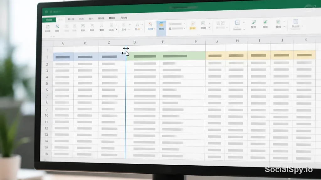
Most people learn column resizing by dragging, and for quick, one-off adjustments, that’s still the right call. Hover your cursor over the border between two column letters at the top of the sheet until it turns into a double-headed arrow, then click and drag left or right.
There’s a faster trick that most casual users never discover: double-clicking that same border instead of dragging it. This triggers AutoFit, which instantly resizes the column to match the width of its longest entry.
- Single drag: Click and hold the column border, drag to desired width, release.
- Double-click AutoFit: Double-click the border between two column headers to auto-size instantly.
- Live width readout: While dragging, Excel shows a tooltip with the exact width in characters and pixels — useful for matching columns precisely.
- Multi-column drag: Select several columns first, then drag any one border; all selected columns resize together to the same width.
Double-clicking a column border is functionally identical to using the “AutoFit Column Width” command from the ribbon — it’s just three seconds faster.
The dragging method works fine when you’re eyeballing it, but it falls apart when you need consistency across a shared template or a report going to a client. That’s where numeric input becomes essential.
Setting an Exact Width With the Column Width Dialog
Excel measures column width in characters of the default font, not pixels or inches, which trips up a lot of users coming from Word or Google Sheets. The default width is 8.43 characters, roughly enough to display 8-9 digits of Calibri 11.
To set a precise width:
- Right-click the column header letter (or select multiple headers) and choose Column Width from the context menu.
- Type a number — for example, 15 for a moderately wide text column, or 3 for a narrow spacer column.
- Click OK, and every selected column snaps to that exact measurement.
You can also do this from the ribbon: Home > Cells > Format > Column Width. It opens the identical dialog box, so use whichever entry point is faster for your workflow.
Why the Character Unit Matters
The character-based unit is a legacy of Excel’s DOS-era roots, and it behaves oddly if you change fonts. A width of “10” in Calibri won’t look the same as “10” in Arial or Times New Roman, because character width varies by typeface.
If you need real-world measurement precision — say, for a printed invoice template — switch to Page Layout view first (View tab > Page Layout). In that view, the Column Width dialog and ruler display measurements in inches or centimeters instead of characters, which is far more intuitive for print design.
Using AutoFit for Instant, Content-Based Sizing
AutoFit is the single most underused feature for column sizing, and it solves the most common complaint: cells showing `####` because numbers don’t fit. Rather than guessing at a width, AutoFit reads every cell in the column and expands it to fit the longest visible entry.
There are three ways to trigger it:
- Double-click any column border, as covered above.
- Select the column(s), then go to Home > Cells > Format > AutoFit Column Width.
- Select the entire sheet with Ctrl+A, then apply AutoFit once to normalize every column simultaneously.
AutoFit has one real limitation worth knowing: it ignores wrapped text height in a strange way and can make columns wider than necessary if a single outlier cell — like a long URL or a stray comment — is buried in an otherwise clean dataset. If you’re building a table with mostly short entries and one abnormally long one, consider truncating or wrapping that entry rather than letting AutoFit blow up the whole column.
This pairs naturally with row height cleanup. Just as columns need matching, tall or inconsistent rows caused by wrapped text often need the same treatment — the process for how to collapse rows in Excel is worth knowing alongside column sizing, since the two frequently get adjusted together on the same messy imported sheet.
Resizing Multiple Columns and Special Cases
Real spreadsheets rarely need just one column adjusted — you’re usually cleaning up an entire imported dataset from a CSV export, a database pull, or a colleague’s file with inconsistent formatting.
Resizing Several Columns at Once
Select column letters by clicking and dragging across the header row (for adjacent columns), or hold Ctrl while clicking individual letters (for non-adjacent columns). Then apply any of the methods above — dragging, double-click AutoFit, or the numeric dialog — and the action applies uniformly to your entire selection.
| Selection Method | How To Do It | Best For |
|---|---|---|
| Adjacent columns | Click letter, drag across headers | Resizing a contiguous block like B:F |
| Non-adjacent columns | Ctrl+click individual letters | Matching widths on scattered columns |
| Entire sheet | Ctrl+A, then Ctrl+A again if needed | Standardizing every column at once |
Handling Merged Cells and Frozen Panes
Merged cells complicate resizing because Excel treats the merged range as a single unit for width calculations — dragging one part of a merged header often distorts the layout underneath it unpredictably. It’s generally cleaner to unmerge, resize, then re-merge if the merge is purely cosmetic.
Frozen panes (View > Freeze Panes) don’t block resizing, but they do split your column headers visually, so make sure you’re grabbing the border in the correct pane if your sheet has a frozen first column. This becomes especially relevant in large tracking sheets where you’ve frozen an ID column and need to widen data columns to the right without accidentally resizing the frozen one.
Setting a Default Width for New Columns
If you’re building a template and want every future column to start at a specific width rather than Excel’s default 8.43, go to Home > Cells > Format > Default Width. This sets the baseline for any column that hasn’t been manually resized yet — handy for standardizing a workbook before you hand it off to a team.
Column Width Pitfalls That Waste Time
Most column-width frustration comes from a handful of predictable mistakes. Recognizing them saves real time on large workbooks.
- Confusing width units after copying between workbooks: If the destination workbook uses a different default font, pasted columns can look narrower or wider than expected even at the “same” numeric width.
- AutoFit ignoring hidden rows: AutoFit calculates width based on visible cells only, so a long entry in a hidden row won’t be accounted for — it can look fine until you unhide that row later.
- Printing surprises: A column that looks perfect on screen may still get cut off or overflow onto a second printed page because print scaling and column width are calculated independently. Always check Print Preview before finalizing a report.
- Locked columns in protected sheets: If a spreadsheet has been shared as read-only, column width changes may be blocked entirely depending on the protection settings, even though the data itself is just view-locked and not width-locked by default — this catches people off guard because they assume formatting is always editable.
- Text overflow vs. truncation confusion: Unformatted text in a too-narrow column will visually overflow into the next cell if that cell is empty, but truncate (show only part of the value) if the next cell has content — same narrow width, two completely different visual results.
A column showing `#####` instead of a number is never a formula error — it’s purely a width problem. Widening the column (manually or via AutoFit) always resolves it instantly.
Understanding that distinction matters because it’s one of the most common support questions in Excel forums, right up there with formulas that display as text instead of calculating. If you’re troubleshooting a sheet where numbers look broken, rule out width issues before digging into anything more complex — related formula troubleshooting steps are covered in Excel formula not calculating, but a `####` display specifically is almost always a sizing fix, not a calculation bug.
Column Width in Broader Spreadsheet Workflows
Column sizing rarely happens in isolation — it’s usually one step in a larger cleanup or formatting pass. Understanding where it fits into a typical workflow helps you batch these tasks efficiently instead of fixing one column at a time across multiple editing sessions.
A typical end-to-end cleanup on an imported dataset looks like this:
- Paste or import raw data into the sheet.
- Select all columns and apply AutoFit as a baseline pass.
- Manually widen or narrow specific columns that need exact, consistent sizing (like ID or date columns).
- Adjust row heights to match, especially where wrapped text is used.
- Apply any text formatting — case corrections, symbol insertions, or combined fields — now that columns are properly sized and easier to read.
- Freeze header rows or key columns for navigation.
- Set sheet protection or read-only status if the file is being distributed.
That fourth and fifth step is where a lot of secondary formatting tasks live. If you’re standardizing inconsistent capitalization from a data export, the same cleanup pass is a natural time to also review how to change text case in Excel, since properly sized columns make it much easier to spot case inconsistencies you’d otherwise miss in a cramped view. Similarly, if you’re merging first and last name fields or combining address components, doing that before your final width pass — rather than after — means you won’t have to re-size columns twice; see [how to combine text from two cells in Excel](https://socialspy.io/how-to combine-text-from-two-cells-in-excel/) for that step.
A Note on Wide Reports and Screen Space
Wider columns aren’t automatically “better formatting” — they eat horizontal screen space fast, especially on financial models or tracking sheets with 15+ columns. A common professional habit is to narrow low-priority columns (like internal notes or flags) to just a few characters wide while keeping primary data columns generously sized, rather than making every column uniform.
For sheets with genuinely too many columns to view comfortably, some users prefer grouping and collapsing sections instead of shrinking width — a technique closely related to expanding and collapsing whole column groups, which is covered in how to expand all columns in Excel. Combining outline grouping with smart width choices is how analysts keep 40-column models navigable without constant horizontal scrolling.
Conclusion
Column width feels like a trivial formatting detail until you’re staring at a sheet full of `#####` symbols or a printed report that cuts off halfway through a column. The core toolkit is small — dragging, double-click AutoFit, and the numeric Column Width dialog — but knowing when to use each one, and how character-based units behave differently from pixels or inches, is what separates a quick fix from a recurring annoyance. Build the habit of running an AutoFit pass immediately after importing data, save manual numeric widths for templates that need consistency, and treat column sizing as the first cleanup step rather than an afterthought, and you’ll spend far less time fighting Excel’s default formatting on every new file you open.
FAQ
This happens when a column is too narrow to display a numeric value in full, and it’s purely cosmetic — the underlying data and any formulas referencing that cell are completely unaffected. Widen the column manually, or double-click the column border to trigger AutoFit, and the correct number will display immediately.
Excel doesn’t have a single command that applies one column width to every sheet in a workbook simultaneously, but you can select multiple sheet tabs at once (Ctrl+click the tabs) before opening the Column Width dialog, and the change will apply to all selected sheets together. Alternatively, set your desired width on one sheet, then use Format Painter or copy the entire column to replicate the formatting elsewhere.
No — column width is purely a display setting and never alters the underlying value, formula, or formatting of the data itself. This is different from text truncation in a program like a plain text field; in Excel, a narrow column simply hides part of the display while the full value remains intact and will show correctly if you widen the column or click into the cell to view it in the formula bar.