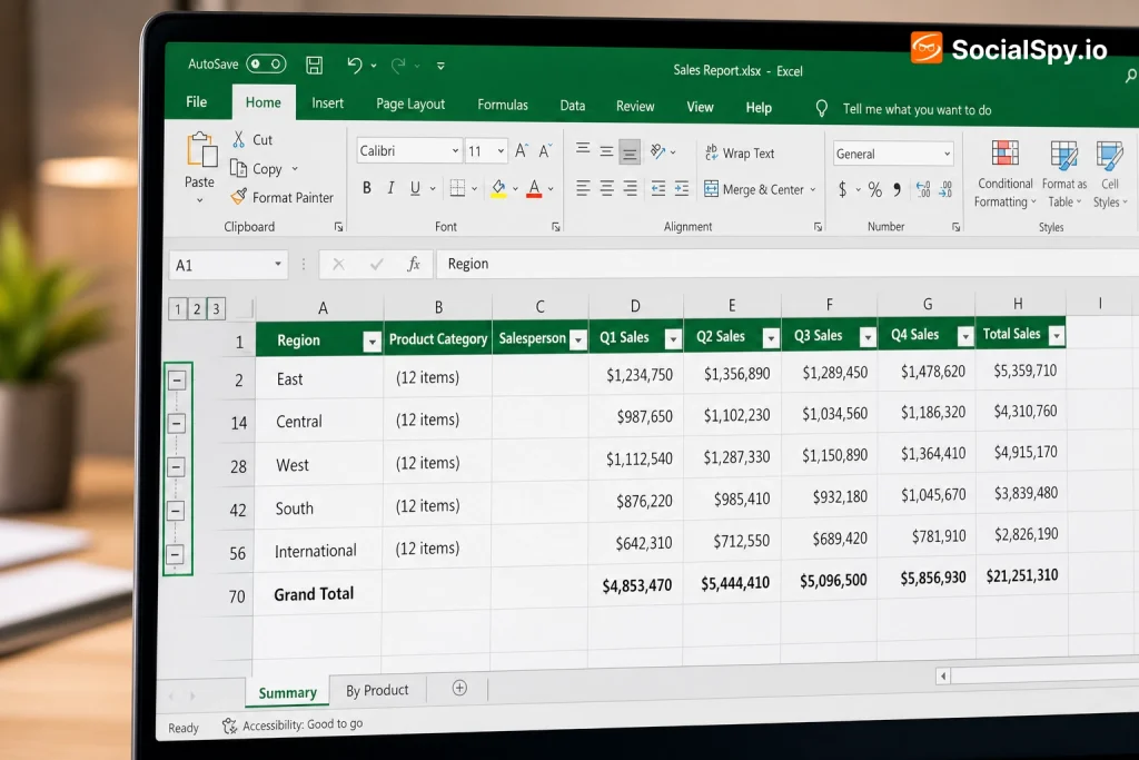
Big spreadsheets get unwieldy fast, especially once you’re scrolling past hundreds of rows just to compare two totals at the top and bottom. Collapsing rows in Excel lets you tuck away the noise and see only what matters, without deleting a single cell of data. This guide covers every method Excel offers in 2026, from quick manual grouping to fully automated outlines that update as your data changes.
The Fastest Way: Manual Row Grouping
The core tool for collapsing rows is Excel’s built-in Group feature, found under the Data tab in the Outline section. It’s different from simply hiding rows because grouping adds a visible, clickable control (a small + or − button) in the left margin, so anyone opening the file knows there’s collapsed content nearby.
Here’s the basic workflow:
- Select the rows you want to collapse — click and drag across the row numbers on the left side of the sheet.
- Go to Data > Outline > Group, or use the keyboard shortcut Shift+Alt+Right Arrow.
- Excel adds a bracket and a minus (−) icon in the margin next to your selected rows.
- Click the minus icon to collapse the rows; click the resulting plus (+) icon to expand them again.
If you want to collapse multiple separate blocks of rows (say, rows 5–10 and rows 20–25), just repeat the process for each block. Excel will show multiple independent collapse controls stacked in the outline margin, and each one operates independently of the others.
A quick sanity check: if Group is greyed out, you likely have a table object or filtered range selected instead of plain rows — convert the table to a range first, or select whole rows rather than just cells.
Auto Outline: Let Excel Detect Structure for You
If your spreadsheet already has subtotals, formulas that reference other rows, or a clear hierarchical layout (like sales data broken into regions with a grand total), Excel can build the grouping structure automatically instead of you doing it row by row.
This lives under Data > Outline > Group dropdown arrow > Auto Outline. Excel scans for patterns — typically rows containing SUM or subtotal formulas — and groups the detail rows beneath each summary row.
- Best for: financial reports, budget sheets, and anything built with the Subtotal feature (Data > Subtotal).
- Not ideal for: raw data dumps with no formulas or summary rows, since Excel has nothing to detect a pattern from.
- Bonus: works with columns too, so wide reports with monthly detail columns collapsing into a quarterly total column benefit the same way.
This is especially useful if you’re already using structured subtotal formulas alongside something like the Profit Margin Formula for Excel, since Auto Outline will recognize those subtotal rows and group the supporting calculation rows beneath them automatically.
Grouping vs. Hiding Rows: What’s the Real Difference
A lot of Excel users default to right-clicking rows and choosing Hide, but that’s a different feature entirely — and it comes with real downsides compared to grouping.
| Feature | Group/Collapse | Hide Rows |
|---|---|---|
| Visible toggle control | Yes (+/− buttons) | No |
| Easy to notice hidden data | Yes | No, easy to miss |
| Reversible in one click | Yes | Requires selecting range and unhiding |
| Works with nested levels | Yes, up to 8 levels | No |
| Good for sharing with others | Yes | Risky, data can be overlooked |
The practical takeaway: use Hide only for rows you genuinely don’t want anyone touching or noticing (like a helper-calculation row). Use Group/Collapse for anything you want a reader to know exists and can expand on demand.
This distinction matters a lot when you’re building dashboards for other people. A collapsed group signals “there’s more detail here if you want it,” while a hidden row can look like the data simply doesn’t exist, which causes confusion in shared files.
Working With Multiple Levels of Nested Groups
Excel supports up to eight levels of nested outline groups, which is what lets you build something like: Country → Region → City → Store, each collapsible independently.
When you have nested groups, Excel displays small numbered buttons (1, 2, 3, etc.) at the top-left of the outline margin. Clicking a number collapses everything down to that level in one click, rather than manually toggling each group.
- Level 1 shows only the grand total row.
- Level 2 expands to show major category subtotals.
- Level 3 and beyond reveal increasingly granular detail rows.
To build nested groups, group your innermost detail rows first, then select a broader range (including the first group) and group again — Excel automatically nests the new group around the existing one. This is the same layered logic used in complex financial models where analysts might also rely on tools covered in guides like Excel Copy Formula to replicate calculations across each nested section without breaking references.
Collapsing Rows Without Grouping: Filters and Manual Hide
Grouping isn’t the only route if you just need a temporary view. Two lighter-weight alternatives exist, and each has a specific use case.
Filtering to Hide Rows Conditionally
Turning your data into a table (Ctrl+T) or applying Data > Filter lets you hide rows based on their values rather than their position. This is ideal when you want to see only, say, rows where “Status = Overdue,” rather than collapsing a fixed block of rows.
- Filters don’t add a +/− toggle; instead, the row numbers themselves turn blue to indicate hidden rows exist.
- Filters are dynamic — as data changes, which rows show or hide updates automatically.
- Filters pair well with Sort, and if you’re regularly reorganizing large data sets, it’s worth learning the newer dynamic array approach in the Sort Excel Function guide, since SORT and FILTER functions together can do a lot of what manual row-hiding used to require.
Manually Hiding Specific Rows
Right-click any selected row number(s) and choose Hide. This is fast but non-obvious to anyone else opening the file, which is why it’s best reserved for personal working files rather than shared reports.
Keyboard Shortcuts and Speed Tips for Power Users
If you collapse and expand rows often, memorizing a handful of shortcuts saves real time over a workday of spreadsheet editing.
- Shift+Alt+Right Arrow — Group selected rows/columns
- Shift+Alt+Left Arrow — Ungroup selected rows/columns
- Ctrl+8 — Toggle the entire outline symbols (+/− buttons) on or off
- Ctrl+9 — Hide selected rows directly
- Ctrl+Shift+9 — Unhide rows within a selection
Another speed tip: click the small outline level buttons (the numbered boxes at the top-left corner, above row 1) to collapse or expand every group on the sheet at once, instead of clicking each minus sign individually. This is the single biggest time-saver once you have more than three or four groups on one sheet.
- To remove all grouping entirely, select the whole sheet (Ctrl+A), then go to Data > Ungroup > Clear Outline.
- Grouping settings are saved with the file, so collapsed states persist the next time the workbook is opened, unless someone expands them and re-saves.
If you’re formatting a report for a wider audience, it also helps to clean up surrounding cosmetic details before you finalize collapsed sections — things like consistent unit labels using How to Insert Degree Symbol in Excel for temperature or measurement data, or consistent capitalization handled via How to Change Text Case in Excel, so the summary rows people see when everything’s collapsed actually look polished.
Common Problems When Collapsing Rows
Even experienced Excel users run into a few recurring snags with grouping. Knowing these in advance saves troubleshooting time later.
“Group” button is greyed out: This almost always means you’re working inside an Excel Table (the blue/green banded style from Ctrl+T) or a PivotTable, neither of which supports manual row grouping the same way. Convert the table to a normal range first (Table Design > Convert to Range).
- Groups disappear after sorting: Outline groups are tied to row position, not content, so sorting data after grouping breaks the structure. Always group after your data is finalized and sorted.
- Formulas break when collapsing: Collapsing doesn’t delete or move data, so formulas referencing collapsed rows keep working fine — but double-check any formula that used to reference a visible range assumption, like conditional formatting based on visible cells only.
- Can’t collapse just one row: Grouping needs at least two adjacent rows selected; a single row can only be hidden, not grouped, since there’s nothing to summarize into a toggle.
- Nested groups collapse together unexpectedly: If you select too broad a range when grouping, you may accidentally nest nest a nest a level higher than intended — check the outline numbers at the top-left to confirm your levels look right.
Conclusion
Collapsing rows is one of those Excel skills that pays off disproportionately to how simple it is — a two-second Group action can turn a 500-row mess into a clean, presentable three-line summary that any stakeholder can expand if they want the details. The key distinction to remember is that grouping is for structured, shareable collapsibility, while hiding and filtering serve narrower, more situational purposes. Once you’ve built the habit of grouping subtotal sections as you build a report — rather than trying to retrofit it later — it becomes as automatic as applying bold text or adjusting column widths.
FAQ
Select the entire worksheet with Ctrl+A, apply Group under the Data tab if you haven’t already grouped sections, then click the lowest-numbered outline level button (usually “1”) in the top-left corner of the sheet to collapse every group simultaneously.
Row grouping isn’t supported inside Excel Tables or PivotTables because their structure is managed differently from regular ranges; convert the table to a normal range first via Table Design > Convert to Range, then apply Group as usual.
No, collapsing only visually hides rows behind a clickable +/− toggle — all data, formulas, and formatting remain fully intact and instantly recoverable by clicking the plus icon, unlike deleting rows which permanently removes content.