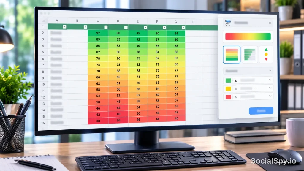
Conditional formatting is one of those Excel features that separates spreadsheets people actually understand from ones that require a translator. Instead of squinting at rows of numbers, you let color, icons, and bars do the heavy lifting so patterns jump out instantly. This guide walks through exactly how to set it up in Excel 2026 (Microsoft 365), what the common pitfalls are, and how to build rules that don’t fall apart the moment someone sorts a column.
The Basics: Applying Your First Rule
Every conditional formatting rule starts the same way: select a range, then tell Excel what condition triggers the formatting. The feature lives under Home > Conditional Formatting on the ribbon, and it’s been in roughly the same spot since Excel 2007.
Here’s the fastest path for a beginner rule:
- Highlight the cell range you want to format (e.g., B2:B50).
- Click Home > Conditional Formatting.
- Choose Highlight Cells Rules for simple comparisons (greater than, less than, between, duplicate values).
- Pick a preset color style or click Custom Format to set your own fill, font, or border.
- Click OK and watch the range update in real time.
For quick visual analysis, Excel’s built-in presets cover most everyday needs:
- Color Scales — shades cells on a gradient (great for heat-map-style sales or temperature data)
- Data Bars — draws a mini bar chart inside each cell, ideal for comparing magnitudes at a glance
- Icon Sets — adds arrows, flags, or traffic-light circles based on value tiers
- Top/Bottom Rules — flags the top 10 items, bottom 10%, or above/below average
Analysts who work with large financial models tend to favor Data Bars over Color Scales for a simple reason: bars communicate relative magnitude faster than color gradients, which some viewers interpret inconsistently.
Formula-Based Rules: The Real Power Move
Presets are fine for simple cases, but the real leverage comes from “Use a formula to determine which cells to format.” This option, buried inside New Rule, lets you write any logical test Excel can evaluate — which means almost anything.
To get there: Home > Conditional Formatting > New Rule > Use a formula to determine which cells to format. You then type a formula that returns TRUE or FALSE, and Excel applies your chosen format whenever it evaluates to TRUE.
A few formulas that come up constantly in real spreadsheets:
- `=B2>100` — highlights any cell in the range greater than 100
- `=$C2=”Overdue”` — highlights an entire row based on a status column
- `=B2<AVERAGE($B$2:$B$50)` — flags values below the dataset average
- `=COUNTIF($A$2:$A$50,A2)>1` — flags duplicate entries
- `=WEEKDAY(A2)=1` — highlights Sundays in a date column
The trick most people miss: relative vs. absolute references decide whether the rule applies uniformly or shifts per cell. Drop a `$` in front of a column or row letter to lock it, and leave it off to let it adjust automatically as Excel walks through the range — this is the exact mechanism behind rules that compare one column against another, which is covered in more depth in Cell Conditional Formatting Based on Another Cell.
Formatting Based on Another Cell or Row
Highlighting a value based on its own contents is easy. Highlighting an entire row based on a value in just one column is where most people get stuck, because it requires understanding how Excel anchors references across a selected range.
Here’s the standard approach for shading a full row when a status column says “Late”:
- Select the full data range, e.g., A2:F200.
- New Rule > Use a formula to determine which cells to format.
- Enter `=$D2=”Late”` (assuming column D holds status).
- Set your fill color, click OK.
The `$D` locks the column reference so it never shifts, while the row number `2` stays relative so it adjusts row by row down the selection. This single-dollar-sign pattern is arguably the most useful trick in all of conditional formatting, and it’s worth memorizing rather than looking up every time.
Common Row-Highlighting Use Cases
- Highlighting overdue invoices based on a due-date column
- Shading rows where a budget variance exceeds a threshold
- Flagging inventory rows where stock falls below a reorder point
- Marking rows where a checkbox/status cell equals “Complete”
Managing, Editing, and Cleaning Up Rules
Conditional formatting rules pile up fast, especially in shared workbooks where multiple people have added their own highlighting over time. Left unmanaged, a workbook can end up with a dozen overlapping rules slowing down recalculation.
The control center is Home > Conditional Formatting > Manage Rules, which opens the Rules Manager. From here you can edit, delete, reorder, and adjust the “Stop If True” checkbox, which prevents lower-priority rules from firing once a higher one matches.
| Task | Where to Find It |
|---|---|
| View all rules on a sheet | Manage Rules > “This Worksheet” dropdown |
| Change rule order/priority | Select rule, use Up/Down arrows |
| Edit an existing formula | Select rule > Edit Rule |
| Delete a single rule | Select rule > Delete Rule |
| Clear all formatting from a range | Conditional Formatting > Clear Rules > Selected Cells |
A frequent source of confusion: rules apply to a specific range, not the whole sheet, unless you explicitly set the range that broad. If a rule seems to “stop working” after adding new rows, it’s usually because the original range never expanded to include them — worth checking before assuming a formula is broken.
Practical Examples for Real Spreadsheets
Conditional formatting earns its keep in specific, repeatable scenarios rather than as decoration. Below are combinations that show up constantly in business spreadsheets.
Budget tracking: Use a formula like `=B2>C2` (actual spend greater than budgeted amount) to turn a cell red, paired with `=B2<=C2*0.9` for green when comfortably under budget. This kind of comparison across two columns is the same logic behind more advanced cell-to-cell comparisons, and if your model also needs running totals, pairing it with the Sum Formula in Excel keeps the whole sheet self-checking.
Sales performance dashboards: Icon Sets with three arrows work well for month-over-month percentage change columns, while Data Bars suit raw revenue figures side by side.
Data cleaning: `=COUNTIF($A:$A,A2)>1` instantly surfaces duplicate customer IDs or SKUs before they cause reporting errors — far faster than scanning manually.
Deadline tracking: `=AND(A2<TODAY(),$C2<>”Done”)` highlights any task whose deadline has passed and isn’t marked complete, combining a date function with a status check in one rule.
Once a sheet gets formatted this heavily, it’s common to want to compress sections for presentation — that’s where How to Collapse Rows in Excel becomes useful, letting you group and hide the highlighted detail rows while keeping summary rows and their formatting visible.
Common Mistakes and How to Avoid Them
Conditional formatting breaks in predictable ways, and almost every “it’s not working” issue traces back to one of these five causes.
- Wrong absolute/relative references — forgetting the `$` (or putting it in the wrong spot) causes rules to shift incorrectly across rows or columns.
- Range doesn’t include new data — pasted or inserted rows outside the original range simply won’t get formatted.
- Format Painter copies rules unexpectedly — using Format Painter can duplicate conditional rules onto cells where they don’t belong, cluttering the Rules Manager.
- Conflicting rules with no priority set — multiple rules targeting the same cells without “Stop If True” can produce unpredictable results.
- Formula referencing the wrong first cell — the formula should always reference the top-left cell of the selected range; get this wrong and every row after the first is off by one.
A quick sanity check: if a formula-based rule works on row 2 but looks wrong by row 15, the issue is almost always a missing or misplaced `$` in the reference — not a bug in Excel.
Another underrated issue: conditional formatting can visually clash with manually applied formatting, like when someone has already widened columns or set fonts by hand. If a dashboard’s columns look cramped once bars or icons are added, adjusting column widths afterward — see How to Modify Column Width in Excel — usually fixes the layout without touching the rules themselves.
Conclusion
Conditional formatting is less about memorizing menu paths and more about understanding one concept: Excel is constantly asking “does this cell make a formula TRUE?” and reformatting based on the answer. Once that clicks, presets like Color Scales and Data Bars become quick wins, while formula-based rules — especially the anchored-reference trick for full-row highlighting — become tools you reach for in nearly every workbook. The skill compounds well too: the same reference logic used here shows up in lookup formulas, data validation, and even chart formatting elsewhere in Excel. Spend twenty minutes actually testing formulas on a scratch sheet, and conditional formatting stops being a mysterious ribbon button and becomes one of the most reliable ways to make a spreadsheet self-explanatory.
FAQ
Not directly through the standard dialog for cross-sheet references in older Excel versions, but in current Excel 2026 (Microsoft 365), formulas in conditional formatting rules can reference other sheets as long as the referenced range is in the same workbook. The safest approach is often to bring the comparison value into a helper column on the same sheet first, then reference that.
Regular Copy/Paste usually carries formatting rules along with it, but Paste Special options like “Values Only” strip formatting entirely, including conditional rules. If formatting vanishes after pasting, check whether Paste Special was used, and reapply the rule to the new range if needed.
Yes, especially with many formula-based rules across large ranges, since Excel recalculates every rule on every recalculation cycle. Trimming ranges to only the cells that need formatting, consolidating overlapping rules, and using “Stop If True” where appropriate all help keep large workbooks responsive.