Every spreadsheet user eventually hits the same wall: you type a formula, hit Enter, and instead of a calculated result, you get the formula text staring back at you, or worse, a value that never updates. It’s one of the most common Excel support questions in 2026, and it usually comes down to one of about eight root causes. This guide walks through each one with the exact fix, so you can stop guessing and get back to working.
Check Your Calculation Mode First
The single most common culprit is a setting most people never touch on purpose: Calculation Options. Excel has three modes — Automatic, Automatic Except for Data Tables, and Manual — and it’s shockingly easy to flip into Manual mode by accident, especially if you’ve opened a workbook someone else built with heavy formula loads.
When a workbook is in Manual mode, formulas only recalculate when you explicitly force them to. That means you can change an input cell, watch nothing happen, and reasonably assume something is broken when nothing actually is.
Here’s how to check and fix it:
- Go to the Formulas tab on the ribbon.
- Click Calculation Options in the Calculation group.
- Select Automatic if it’s currently set to Manual.
- Press F9 to force an immediate recalculation of the entire workbook.
- Use Shift+F9 to recalculate only the active worksheet, or Ctrl+Alt+F9 for a full forced recalculation including hidden dependencies.
Large financial models with tens of thousands of formulas are often deliberately set to Manual to prevent Excel from freezing during data entry. If you’ve inherited a workbook like this, that’s normal — just remember to hit F9 before trusting any number.
Manual mode is sticky at the application level in some Excel versions, meaning it can carry over between files you open in the same session. That’s why a workbook that calculated fine yesterday might suddenly seem broken today, even though you never touched a single formula.
The Cell Is Formatted as Text, Not Formula
This is the classic “typed a formula, got the formula back as text” problem, and it trips up even experienced users. If a cell was formatted as Text before you typed `=SUM(A1:A10)` into it, Excel treats the entire entry as a literal string instead of an instruction to calculate.
You’ll know this is happening if:
- The formula is left-aligned instead of right-aligned (numbers and formula results default to right-aligned).
- There’s a small green triangle in the upper-left corner of the cell with a warning about “Number Stored as Text” or “Formula in Text Format.”
- Clicking the cell shows the formula bar contains the exact text you typed, but the cell just displays it flatly with no calculation.
The fix requires more than just changing the format — Excel needs to be told to re-parse the entry:
- Select the affected cell or range.
- Go to Home > Number and change the format from Text to General or Number.
- Click into the formula bar for each affected cell and press Enter again (this forces re-evaluation).
- For multiple cells at once, select the range, use Data > Text to Columns, and click Finish without changing any settings — this is a well-known workaround that forces Excel to reinterpret every cell in the selection.
If you’re regularly combining data from two sources — say, merging names or IDs pulled from different systems — text formatting issues compound fast, which is a big reason spreadsheet builders lean on functions covered in guides like How to Combine Text From Two Cells in Excel rather than manual paste jobs that drag inconsistent formatting along with them.
Show Formulas Mode Is Accidentally Turned On
If every single formula in your worksheet is displaying as text instead of a result — not just one cell, but the whole sheet — you’ve probably toggled Show Formulas mode without realizing it.
This mode is genuinely useful for auditing a workbook, but it’s controlled by a keyboard shortcut that’s easy to hit by accident:
- The shortcut is Ctrl+` (Ctrl plus the grave accent key, usually just left of the “1” key).
- It’s a toggle, so pressing it again turns it off.
- You can also check it manually under Formulas > Show Formulas.
How to tell the difference from the text-formatting issue
| Symptom | Show Formulas Mode | Text-Formatted Cells |
|---|---|---|
| Scope | Affects entire sheet at once | Usually isolated cells or ranges |
| Toggle | Ctrl+` fixes it instantly | Requires reformatting + re-entry |
| Column width | Columns often auto-widen to show formula text | No width change |
| Green triangle warning | Not present | Usually present |
If it’s a whole-sheet issue, check Show Formulas before you touch anything else. It’s a thirty-second fix and saves you from reformatting cells that were never broken in the first place.
Circular References and Iterative Calculation Settings
Sometimes a formula doesn’t calculate because Excel has flagged it as part of a circular reference — a formula that, directly or indirectly, refers back to its own cell. Excel will show a warning dialog the first time this happens, but if you dismiss it and keep working, the cell often just displays 0 or freezes at whatever value it last held.
Common causes include:
- A `SUM` range that accidentally includes the total cell itself.
- Two cells referencing each other (A1 references B1, B1 references A1).
- Cross-sheet formulas that create a loop across multiple tabs without you realizing it.
Excel actually supports intentional circular references through iterative calculation, which is useful for certain financial models (like circular interest calculations), but it’s off by default:
- Go to File > Options > Formulas.
- Check Enable iterative calculation under Calculation options.
- Set Maximum Iterations (default 100) and Maximum Change (default 0.001).
For most everyday spreadsheets, though, a circular reference is a mistake, not a feature. Use Formulas > Error Checking > Circular References to jump straight to the offending cell instead of hunting through the sheet manually.
Formula Errors, Broken References, and Volatile Function Overload
Not every “not calculating” complaint is actually a calculation setting problem — sometimes the formula is calculating just fine, but returning an error value that looks like a freeze. Recognizing which error you’re looking at narrows down the fix immediately.
- #REF! — A cell the formula depends on was deleted. Rebuild the reference rather than trying to “fix” it in place.
- #NAME? — Excel doesn’t recognize a function name, often from a typo or from using a function that doesn’t exist in your Excel version (common with newer dynamic array functions on older installs).
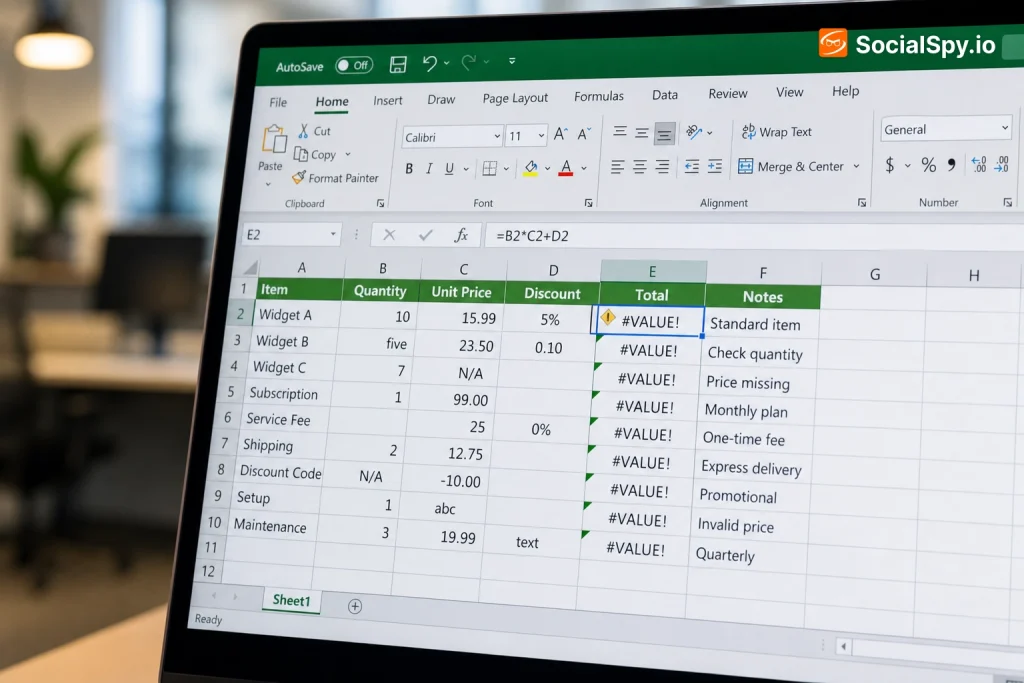
- #VALUE! — A formula is trying to do math on text, frequently caused by the text-formatting issue described above.
- #N/A — Usually from `VLOOKUP`, `INDEX/MATCH`, or `XLOOKUP` when the lookup value genuinely isn’t in the range.
- #DIV/0! — Division by zero or by an empty cell, common in ratio and percentage calculations.
That last one shows up constantly in business spreadsheets — anyone building a pricing or reporting sheet, like the calculations in a Profit Margin Formula for Excel setup, will run into #DIV/0! the moment a revenue cell is blank rather than zero, so wrapping formulas in `IFERROR()` is worth doing proactively rather than reactively.
There’s also a performance-related version of “not calculating”: workbooks stuffed with volatile functions like `NOW()`, `TODAY()`, `RAND()`, `OFFSET()`, and `INDIRECT()` recalculate on every single change anywhere in the workbook, not just when their own inputs change. In large files with thousands of these, Excel can appear to hang or lag so badly that it feels like calculation has stopped, when it’s actually just overwhelmed.
- Replace `OFFSET()` with `INDEX()` where possible — INDEX is not volatile.
- Limit `NOW()` and `TODAY()` usage to a single cell that other formulas reference, rather than repeating the function everywhere.
- Check File > Options > Advanced > Formulas for the “enable multi-threaded calculation” setting, which is on by default but worth confirming on older hardware.
Hidden Characters, Leading Apostrophes, and Copy-Paste Corruption
A sneaky cause of formula failure is invisible characters that got dragged in from pasted data — things like non-breaking spaces from a web page, or a stray leading apostrophe that forces a cell into text mode even though it looks completely normal.
A leading apostrophe (`’`) is Excel’s built-in “force text” character. It’s invisible in the cell display but visible in the formula bar, and it will silently turn `=A1+A2` into inert text if it precedes the equals sign.
Quick ways to spot and clean this up:
- Click the cell and look at the formula bar — if you see `’=SUM(…)` with an apostrophe before the equals sign, that’s your problem.
- Use `=CLEAN(A1)` combined with `=TRIM(A1)` to strip non-printing characters and extra spaces from imported data before referencing it in calculations.
- When copying formulas across a range, use Paste Special > Formulas instead of a plain paste to avoid dragging along formatting quirks from the source cells — this is one of the most common mistakes covered in a deeper breakdown of Excel Copy Formula techniques.
If you’re pulling data from a database export, a PDF conversion, or a web scrape, run it through `CLEAN()` and `TRIM()` as a default first step. It costs one extra column and saves an hour of confused troubleshooting later.
Workbook Structure Issues That Mimic Calculation Failure
Occasionally the workbook itself is structured in a way that makes formulas appear broken when they’re technically working exactly as written. This is less about settings and more about layout mistakes that are easy to make in large, evolving spreadsheets.
- Merged cells breaking ranges — A `SUM` or `AVERAGE` formula that spans merged cells can return unexpected results because Excel only stores the value in the top-left cell of a merge.
- Filtered or hidden rows skewing totals — `SUBTOTAL()` respects filters, but plain `SUM()` does not, so totals can look “stuck” when rows are hidden by a filter rather than deleted.
- Grouped/collapsed sections hiding the actual source cells — if you’ve grouped and collapsed rows to clean up a report, it’s worth double-checking that summary formulas still point to the right cells underneath; the mechanics of this are covered well in How to Collapse Rows in Excel, which also explains how outline levels interact with formula ranges.
- Sorting that breaks relative references — using a basic sort on a range that includes formulas with relative cell references can shuffle the formulas out of alignment with their intended data; functions covered in a guide to the Sort Excel Function explain how dynamic array sorting avoids this specific trap.
None of these throw an error message. They just quietly produce a number that’s technically calculated but functionally wrong, which is arguably worse than an outright freeze because it’s harder to catch in a quick glance.
Conclusion
“Excel formula not calculating” is rarely a single, mysterious bug — it’s almost always one of a handful of well-documented behaviors that Excel is technically doing on purpose, just not the way you expected. The fastest diagnostic path is to check Calculation Options first, since it explains the widest range of symptoms with the least effort, then work down through cell formatting, Show Formulas mode, circular references, and hidden characters in that order.
Building the habit of pressing Ctrl+` to audit formulas visually, wrapping risky calculations in `IFERROR()`, and running `CLEAN()`/`TRIM()` on any imported data will prevent the vast majority of these issues before they ever show up. Spreadsheets that look broken are usually just spreadsheets that are telling you something specific — you just have to know which of the eight things to listen for.
FAQ
This almost always means the cell is formatted as Text rather than General or Number, or that Show Formulas mode (toggled with Ctrl+`) is switched on for the whole sheet. Reformat the cell and re-enter the formula, or press Ctrl+` again to toggle formula display off.
The workbook’s Calculation Options are almost certainly set to Manual instead of Automatic. Go to Formulas > Calculation Options and switch it to Automatic, then press F9 once to force an immediate full recalculation.
These are legitimate calculated results, not calculation failures — #VALUE! means the formula is trying to do math on text (often from a formatting issue), and #DIV/0! means it’s dividing by zero or an empty cell. Wrapping the formula in IFERROR() lets you display a blank or custom message instead of the raw error.