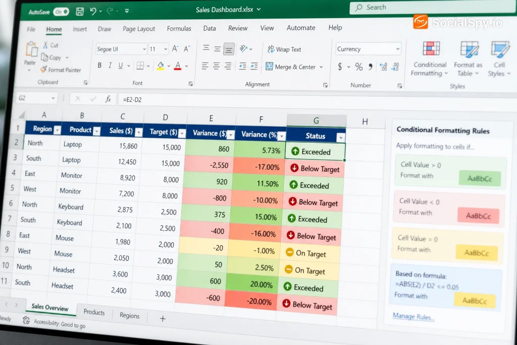
Spreadsheets get a lot smarter the moment one cell can react to what’s happening in another. Instead of manually color-coding rows every time a budget shifts or a deadline slips, you set a rule once and let the sheet police itself. This guide walks through exactly how to build cross-cell conditional formatting in both Excel and Google Sheets, plus the formulas that actually hold up in real spreadsheets.
Why Cross-Cell Formatting Matters More Than Basic Rules
Most people’s first experience with conditional formatting is a simple built-in rule: highlight cells greater than 50, or flag duplicates. That works fine when a cell needs to judge itself. It falls apart the moment your logic depends on a different cell entirely.
Think about a shipping tracker where column C should turn red if the date in column B has already passed. Or a sales dashboard where a rep’s name in column A should bold itself if their revenue in column D missed quota. Neither of these is a “format this cell based on its own value” problem — they’re relational.
- Inventory sheets: flag a product row if stock in one cell drops below the reorder threshold in another
- Project trackers: color a task if its due date cell is earlier than today’s date
- Budgets: highlight actual spend cells that exceed the budgeted amount in an adjacent cell
- HR rosters: shade a name if a certification expiration date is within 30 days of today
Industry spreadsheet trainers consistently note that formula-based conditional formatting is the single most underused feature in Excel and Google Sheets, largely because the “use a formula” option is buried a click deeper than the preset rules.
Once you understand the pattern, it applies to dozens of everyday tracking problems without a single macro or script.
The Core Mechanics in Excel
Excel’s conditional formatting engine is powerful but unforgiving about reference types. Get the dollar signs wrong and the rule either applies to the wrong cells or does nothing at all.
Setting Up the Rule
- Select the range you want to format — say, C2:C20, where C is “Actual Spend”
- Go to Home > Conditional Formatting > New Rule
- Choose “Use a formula to determine which cells to format”
- Enter a formula referencing the first row of your selection, such as `=C2>B2` (where B is “Budgeted Amount”)
- Click Format, choose a fill color or font style, then OK
The critical detail is that Excel applies the formula relative to the top-left cell of your selected range, then adjusts automatically as it moves down. That’s why you write the formula for row 2 only, not for every row.
Reference Types That Actually Matter
| Reference Style | Example | Behavior |
|---|---|---|
| Relative | `C2>B2` | Row and column shift as it copies down/across |
| Column-locked | `$C2>$B2` | Column stays fixed, row shifts (typical for column-based rules) |
| Fully absolute | `$C$2>$B$2` | Nothing shifts — everything compares to one fixed cell |
For most “compare this row to that row” scenarios, you want the row number to move but not be locked, and often the column locked with a `$` sign if the formula will also be applied across multiple columns. Get this wrong and you’ll see the classic symptom: row 5 highlighting based on row 2’s data.
A common real-world formula for a project tracker looks like this:
`=AND($E2<TODAY(), $F2<>”Complete”)`
That flags any row where the due date (column E) has passed and the status (column F) isn’t marked complete — a two-cell dependency wrapped in one rule.
The Core Mechanics in Google Sheets
Google Sheets handles the same concept with slightly different menu names but nearly identical formula logic, which matters if your team splits time between the two platforms.
Step-by-Step in Sheets
- Select your range, e.g., A2:D20
- Click Format > Conditional formatting
- Under “Format rules,” change the dropdown to “Custom formula is”
- Enter something like `=$D2<$C2` to flag rows where actual (D) falls short of target (C)
- Choose a formatting style in the panel and hit Done
Google Sheets applies the custom formula to every cell in the selected range independently, evaluating it as if that cell were the anchor — which is why the `$` column lock is almost always necessary when the rule needs to look at one specific column while formatting a different one.
A Practical Example: Highlighting Overdue Tasks
Say column B has due dates and you want to highlight the entire row (columns A through E) when a task is overdue:
- Select range A2:E100
- Custom formula: `=$B2<TODAY()`
- Format: light red fill
Because the column is locked on B but the row isn’t, Sheets correctly checks B2 for row 2, B3 for row 3, and so on, while formatting the whole row each time. This single-rule, whole-row technique is one of the most requested tricks in spreadsheet forums because it turns a flat table into something that visually manages itself.
Advanced Formulas Worth Stealing
Once the basic pattern clicks, the real value comes from combining functions inside the conditional formatting formula bar. These aren’t exotic — they’re the ones that show up constantly in real business sheets.
- Comparing to a moving average: `=C2>AVERAGE($C$2:$C$50)*1.2` flags any value 20% above the column average
- Cross-sheet comparison: `=Sheet1!B2<>Sheet2!B2` highlights mismatches between two tabs during reconciliation
- Text-based matching: `=EXACT($A2,$B2)=FALSE` flags rows where two name fields don’t match exactly (case-sensitive)
- Date proximity: `=AND($C2-TODAY()<=7,$C2-TODAY()>=0)` highlights anything due within the next week
- Nested logic: `=IF($E2=”High”,$F2<5,$F2<10)` applies different thresholds depending on a priority label
That last one is worth pausing on. Conditional formatting formulas support `IF` statements just like regular cells do, which means the threshold itself can depend on another cell’s value — not just a simple comparison. That’s how you build a single rule that behaves differently for “High” priority rows versus everything else, instead of stacking five separate rules.
Common Mistakes That Break the Rule
Almost every conditional formatting failure traces back to one of a handful of predictable errors. Knowing them in advance saves the debugging headache.
Reference Lock Mistakes
The single most common issue is forgetting that conditional formatting formulas behave like they’re being “dragged” across the entire selected range. If you lock a reference that should move, every row ends up comparing against the same cell instead of its own neighbor.
Range Selection Order
In Excel specifically, the formula is evaluated relative to the active cell in the selection — which is usually the top-left cell, but not always if you selected the range by dragging from a different corner. If a rule seems to be off by one row or column, check which cell was active when you built the selection.
Format Painter Overwrites
Copying formatting with the Format Painter or paste-special can strip or duplicate conditional formatting rules unexpectedly. It’s safer to use Conditional Formatting > Manage Rules and adjust the “Applies to” range directly rather than copy-pasting cells that contain rules.
Rule Priority Conflicts
Both platforms let you stack multiple rules on the same range, and they evaluate top to bottom (Excel) or top to bottom in the rules list (Sheets), stopping at the first match unless “stop if true” is unchecked. A common bug: a broad rule sitting above a specific one silently blocks the specific rule from ever firing.
A frequent troubleshooting tip from spreadsheet consultants: if a conditional format “isn’t working,” open Manage Rules first — in roughly half of reported cases, the rule is firing correctly but a different rule higher in the list is winning the conflict.
Excel vs. Google Sheets: Where They Diverge
The formula syntax is nearly identical between the two, but there are real functional differences worth knowing before you standardize a team template.
| Feature | Excel | Google Sheets |
|---|---|---|
| Formula bar location | Home > Conditional Formatting > New Rule | Format > Conditional formatting > Custom formula |
| Real-time collaboration | Requires OneDrive/SharePoint sync | Native, instant multi-user editing |
| Cross-sheet references in rules | Supported, less commonly used | Fully supported, common in reconciliation sheets |
| Rule limit per sheet | Practically unlimited (performance may lag) | Soft practical limits before slowdown |
| Mobile app rule creation | Limited editing on mobile | Also limited, view-only recommended |
If your team is already leaning into shared, browser-based work, this is one more reason spreadsheets increasingly live alongside broader cloud based productivity apps rather than as isolated desktop files. A conditional formatting rule built once in a shared Sheets file updates the visual logic for everyone viewing it in real time, which isn’t quite as instantaneous with Excel unless the whole team is synced through the same cloud storage.
Real-World Use Cases Worth Copying
Beyond the generic examples, here are specific setups that show up constantly in operational spreadsheets across sales, ops, and finance teams in 2026.
- Sales pipeline aging: Highlight a deal row red if `TODAY() – $LastContactDate > 14`, forcing reps to notice stalled deals without a separate report
- Budget variance: Format actual-spend cells with a gradient based on how far they exceed the budget cell in the adjacent column, using a formula like `=($C2-$B2)/$B2>0.1`
- Certification compliance: Flag employee rows where an expiration date cell falls within 30 days of today, paired with a second rule for already-expired dates in a stronger color
- Inventory reorder points: Compare current stock cell against a reorder threshold cell stored elsewhere on the sheet, so changing the threshold instantly updates every highlighted row
- Grade thresholds: Compare a student’s score cell against a passing-grade cell that a teacher can adjust once per class without rewriting each student’s row
The common thread across all five: the threshold or comparison value lives in its own cell rather than being hardcoded into the formula. That’s the real payoff of cross-cell conditional formatting — change one input cell, and every dependent formatted cell across the sheet updates instantly without touching the rule itself.
Conclusion
Cell conditional formatting based on another cell isn’t a niche trick — it’s the difference between a spreadsheet that just stores numbers and one that actively flags what needs attention. The mechanics are nearly identical in Excel and Google Sheets: pick “use a formula,” reference the comparison cell with the right mix of relative and absolute signs, and let the range do the rest. Once the reference-locking pattern clicks, you can chain in `IF`, `AND`, `TODAY()`, and `AVERAGE()` to build rules that would otherwise require a formula column and a separate glance. Start with one rule on one range, confirm it behaves across every row before adding a second, and the whole system scales cleanly instead of turning into a tangle of conflicting formats.
FAQ
Yes, both Excel and Google Sheets support cross-sheet references inside conditional formatting formulas, such as `=Sheet2!B2>100`. Just be aware that Excel requires the referenced sheet to exist in the same workbook, and very large cross-sheet rule sets can slow down recalculation on bigger files.
This almost always comes down to reference locking — if you used a fully absolute reference like `$B$2` instead of `$B2`, every row in your range is comparing against that same fixed cell instead of its own row. Fix it by removing the dollar sign in front of the row number so the reference shifts down naturally as the rule applies to each row.
Neither Excel nor Google Sheets enforces a hard numeric cap, but performance degrades noticeably once you stack hundreds of formula-based rules across large ranges, especially with volatile functions like `TODAY()` or `NOW()` recalculating constantly. For most business spreadsheets, consolidating logic into fewer, smarter formulas using `AND`, `OR`, and `IF` performs far better than dozens of narrow single-condition rules.